Exploring Red Wine Quality Through Data Science

Supervisor: Prof. Garg
Type: Academic Project (Data Science, Machine Learning)

Overview

This project, led by Prof. Garg, aimed to explore the quality of red wine using data science techniques. The objective was to analyze the physicochemical properties of red wine and to determine the best indicators of quality using Regression and Classification Models.

Methodology

The methodology included:

Exploratory Data Analysis (EDA): Conducting an initial analysis to understand the dataset and identify potential relationships.
Data Preparation: Addressing missing values, handling outliers, and implementing feature scaling.
Regression Model Implementation: Employing Random Forest and Gradient Boosting models to predict wine quality.
Classification Model Development: Utilizing a Neural Network using TensorFlow and Keras for quality classification.

Evaluation

The evaluation of the models involved:

Regression Model Assessment: Using metrics like R-squared, RMSE, and MAE for performance evaluation.
Classification Model Analysis: Tracking training and validation loss and accuracy, along with Precision, Recall, and Accuracy metrics.

Key Findings

Identified key physicochemical properties that significantly influence wine quality.
Random Forest and Gradient Boosting models provided insights into the wine quality, with Random Forest showing slightly better performance.
The Neural Network model demonstrated a promising ability to classify wine quality, though constrained by the dataset size.

Personal Contributions

Complete Project Leadership: Oversaw all aspects of the project from data collection to model development and evaluation.
Data Analysis and Preprocessing: Conducted thorough EDA, data cleaning, and preparation for modeling.
Model Development and Optimization: Developed both regression and classification models, focusing on fine-tuning and optimization.
Performance Evaluation: Assessed the models using various metrics and interpreted the results to draw meaningful conclusions.

Conclusion

This project showcased the effectiveness of data science techniques in analyzing and predicting red wine quality. The use of advanced modeling approaches provided valuable insights into the factors influencing wine quality and demonstrated the potential of machine learning in the food and beverage industry.

Project’s Jupyter Notebook

Project’s jupyter notebook can be viewed via this link

Or, you can view the text representation of it as follows:

Exploring Red Wine Quality Through Data Science

You can read more about the Data Science Methodology from this IBM whitepaper by John Rollins

Link for the dataset for context

Business Understanding

The red wine industry shows a recent exponential growth as social drinking is on the rise. Nowadays, industry players are using product quality certifications to promote their products. This is a time-consuming process and requires the assessment given by human experts, which makes this process very expensive. Also, the price of red wine depends on a rather abstract concept of wine appreciation by wine tasters, opinion among whom may have a high degree of variability. Another vital factor in red wine certification and quality assessment is physicochemical tests, which are laboratory-based and consider factors like acidity, pH level, sugar, and other chemical properties. The red wine market would be of interest if the human quality of tasting can be related to wine’s chemical properties so that certification and quality assessment and assurance processes are more controlled.

The goal is to implement Regression Models and Classification Models on the Red Wine Quality Dataset to determine which features are the best quality red wine indicators and generate insights into each of these factors to our model’s red wine quality.

Analytic Approach

Based on the above business understanding one should decide the analytical approach to follow. The approaches can be of 4 types: Descriptive approach (current status and information provided), Diagnostic approach(a.k.a statistical analysis, what is happening and why it is happening), Predictive approach(it forecasts on the trends or future events probability) and Prescriptive approach( how the problem should be solved actually).

Q1. What is the analytical approach that you would take for this project? Why do you think its the right approach?

I would take Descriptive approach as we yet do not know what information are useful and have high impact on our wine quality. We are just presented with the raw data and descriptive approach would enable us to have an understanding of the potential relationships between variables and also helps us to present the data in a more meaningful way. After our analysis is finished, we would do the modellings.

Data Requirements

Q2. What kind of data do we require for predicting the red wine quality and for determining the features that are the best quality red wine indicators?

We need a data which has many features like the physiochemical attributes (acidity, pH level, sugar, etc) so that we would have enough features to play around with to determine the features that are the best quality red wine indicators.

Data Collection

Q3. From where do we get our data?

We get our data from Wine Quality Dataset which is gathered by:

Paulo Cortez, University of Minho, Guimarães, Portugal, http://www3.dsi.uminho.pt/pcortez
A. Cerdeira, F. Almeida, T. Matos and J. Reis, Viticulture Commission of the Vinho Verde Region(CVRVV), Porto, Portugal @2009

and is accessible on UCI ML repository via this link https://archive.ics.uci.edu/ml/datasets/wine+quality

Data Understanding

Link for the dataset https://archive.ics.uci.edu/ml/datasets/wine+quality for context

Q4. From where are red wine samples obtained?

The red wine samples were obtained from the north of Portugal to model red wine quality based on physicochemical tests. The dataset is related to the red variant of Portuguese “Vinho Verde” wine.

Q5. How can knowing the impact of each variable on the red wine quality help businesses(producers, distributors, etc) ?

Knowing the impact of each variable would help businesses(producers, distributors, etc) better assess their production, distribution, and pricing strategy.

Check the shape of data, and the datatypes of the features

Understand the data by carrying out any steps that you think are necessary

import matplotlib.pyplot as plt
import joblib
import pandas as pd
import numpy as np
import seaborn as sns
import warnings
from sklearn.preprocessing import normalize, StandardScaler
warnings.filterwarnings("ignore", category=UserWarning)
warnings.filterwarnings("ignore", category=FutureWarning)
warnings.filterwarnings('ignore', category=DeprecationWarning)
from sklearn.model_selection import train_test_split
from sklearn import svm
from sklearn.metrics import accuracy_score, precision_score, recall_score, classification_report
from sklearn.model_selection import GridSearchCV

wine = pd.read_csv("winequality-red.csv")
wine.head()

	fixed acidity	volatile acidity	citric acid	residual sugar	chlorides	free sulfur dioxide	total sulfur dioxide	density	pH	sulphates	alcohol	quality
0	7.4	0.70	0.00	1.9	0.076	11.0	34.0	0.9978	3.51	0.56	9.4	5
1	7.8	0.88	0.00	2.6	0.098	25.0	67.0	0.9968	3.20	0.68	9.8	5
2	7.8	0.76	0.04	2.3	0.092	15.0	54.0	0.9970	3.26	0.65	9.8	5
3	11.2	0.28	0.56	1.9	0.075	17.0	60.0	0.9980	3.16	0.58	9.8	6
4	7.4	0.70	0.00	1.9	0.076	11.0	34.0	0.9978	3.51	0.56	9.4	5

# The shape of data
print('Number of samples: ', wine.shape[0])
print('Number of features: ', wine.shape[1])

Number of samples:  1599
Number of features:  12

# The datatypes of the features
wine.info()

<class 'pandas.core.frame.DataFrame'>
RangeIndex: 1599 entries, 0 to 1598
Data columns (total 12 columns):
#   Column                Non-Null Count  Dtype  
---  ------                --------------  -----  
0   fixed acidity         1599 non-null   float64
1   volatile acidity      1599 non-null   float64
2   citric acid           1599 non-null   float64
3   residual sugar        1599 non-null   float64
4   chlorides             1599 non-null   float64
5   free sulfur dioxide   1599 non-null   float64
6   total sulfur dioxide  1599 non-null   float64
7   density               1599 non-null   float64
8   pH                    1599 non-null   float64
9   sulphates             1599 non-null   float64
10  alcohol               1599 non-null   float64
11  quality               1599 non-null   int64  
dtypes: float64(11), int64(1)
memory usage: 150.0 KB

From the below table, we can see that the data in our dataset is not distributed well and we have a lot more medium quality wines than the very high or low quality wines.

# understanding the data
print(list(wine.columns))
wine['quality'].value_counts()

['fixed acidity', 'volatile acidity', 'citric acid', 'residual sugar', 'chlorides', 'free sulfur dioxide', 'total sulfur dioxide', 'density', 'pH', 'sulphates', 'alcohol', 'quality']





  681
  638
  199
   53
   18
   10
Name: quality, dtype: int64

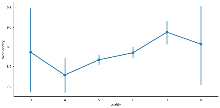
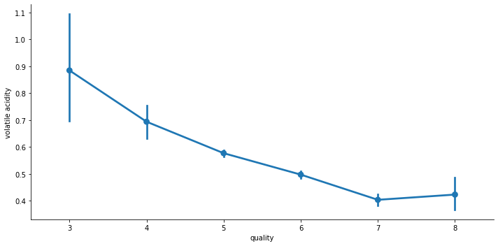
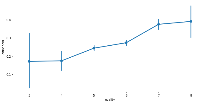
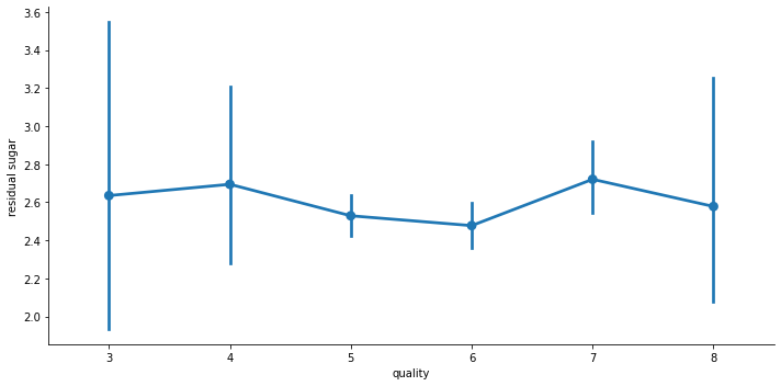
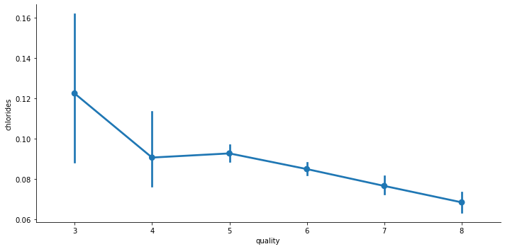
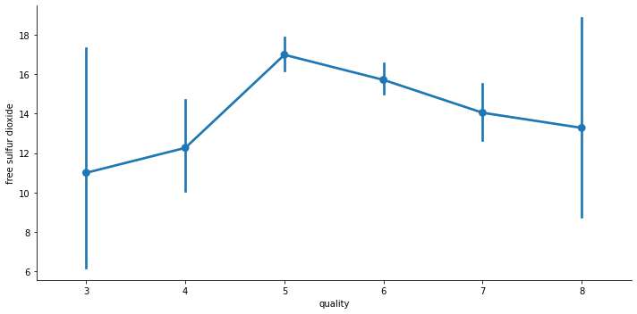
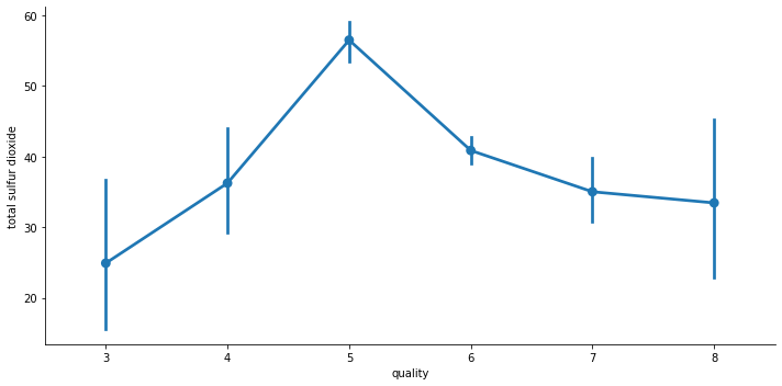
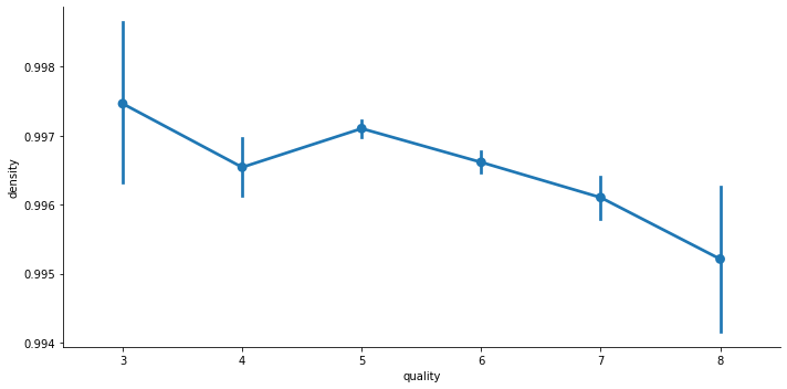
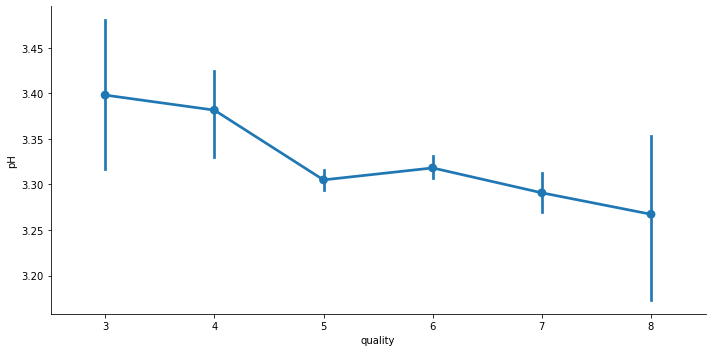
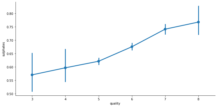
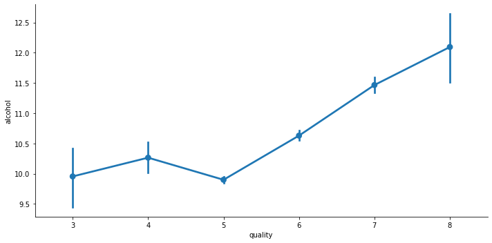
As we can see in the graphs below, generally, when there is low volatile acidity, chlorides, density, and pH, the quality of the wine is higher and with the increase in citric acid, sulphates, and alcohol the quality becomes higher. The residual sugar does not have much of a impact; as we can see in the graph of residual sugar Vs. quality, across different wine qualities, the residual sugar remains the same. The rest of the features have a mixture of behaviours regarding their impact on the quality.

for i, col in enumerate(list(wine.drop('quality', axis=1).columns)):
    plt.figure(i)
    sns.catplot(x='quality', y=col, data=wine, kind='point', aspect=2, )

<Figure size 432x288 with 0 Axes>

png

Data Preparation

Explore the dataset further

TODO

Check for missing values and handle if any

Check for outliers if any and handle them

Implement Correlation heatmap

Check the distribution of data using histograms

Prepare the data for modeling by carrying out any steps that you think are necessary

(masalan feature scaling mitoonim anjam bedim ba standard scalar chon ke az plot e outlier ha mishe fahmid ke scale ashoon aslaaan yeki nist)

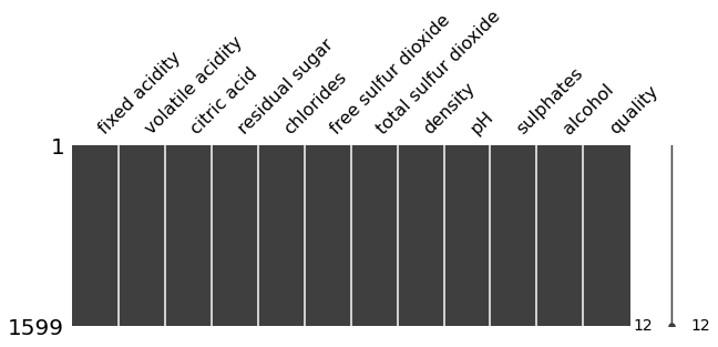
There are no missing values in our dataset.

# Check for missing values and handle if any
import missingno as msno

msno.matrix(wine,figsize=(10,3))

<AxesSubplot:>

png

There are obviously some outliers in our dataset which need to be handled. Also, from this graph we can see that the features are not on the same scale so we have class imbalance which we will need to handle using feature scaling.

# Check for outliers if any and handle them
fig = plt.figure(figsize = (15,8))
wine.drop(['quality'], axis=1).boxplot(grid=False)

<AxesSubplot:>

png

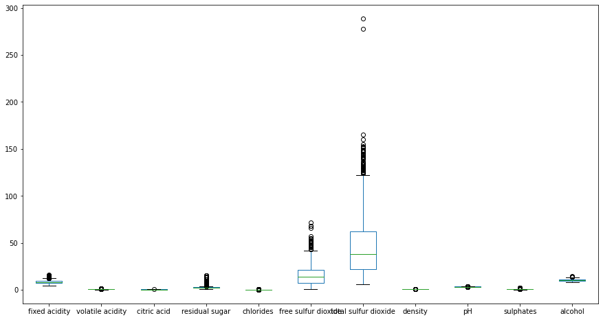
As the number of outliers detected in total are more than 25% of our dataset, then not dropping them would be more reasonable. We will try to cap and floor the outliers by the 10th and 90th percentile.

# handling the outliers present

df = wine.copy()

Q1 = df.quantile(0.25)
Q3 = df.quantile(0.75)
IQR = Q3 - Q1

# This part of the code is taken from StackOverflow
df = df[~((df < (Q1 - 1.5 * IQR)) |(df > (Q3 + 1.5 * IQR))).any(axis=1)]

print("Number of outliers detected %d" % (len(wine) - len(df)))
print("Proportion of outliers to the whole dataset is %f" % ((len(wine) - len(df))/len(wine)))

Number of outliers detected 420
Proportion of outliers to the whole dataset is 0.262664

# handling the outliers present

df = wine.copy()

tenth_percentile = df.quantile(0.1)
ninetieth_percentile = df.quantile(0.9)

df = df.drop(['quality'], axis=1).clip(tenth_percentile, ninetieth_percentile, axis = 1)

# savng the dataframe for future use
df = df.assign(quality = wine['quality'])
wineMod = df

wineMod.head()

	fixed acidity	volatile acidity	citric acid	residual sugar	chlorides	free sulfur dioxide	total sulfur dioxide	density	pH	sulphates	alcohol	quality
0	7.4	0.700	0.010	1.9	0.076	11.0	34.0	0.9978	3.51	0.56	9.4	5
1	7.8	0.745	0.010	2.6	0.098	25.0	67.0	0.9968	3.20	0.68	9.8	5
2	7.8	0.745	0.040	2.3	0.092	15.0	54.0	0.9970	3.26	0.65	9.8	5
3	10.7	0.310	0.522	1.9	0.075	17.0	60.0	0.9980	3.16	0.58	9.8	6
4	7.4	0.700	0.010	1.9	0.076	11.0	34.0	0.9978	3.51	0.56	9.4	5

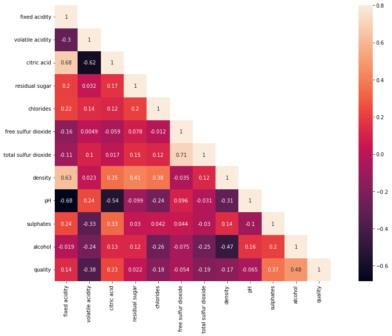
The correlation heatmap shows that there is no feature that is highly correlated (correlation > 0.5) with the quality of the wines.

# Implement Correlation heatmap

corrMatt = wineMod.corr()
mask = np.array(corrMatt)
mask[np.tril_indices_from(mask)] = False
fig,ax= plt.subplots()
fig.set_size_inches(20,10)
sns.heatmap(corrMatt, mask=mask,vmax=.8, square=True,annot=True)

<AxesSubplot:>

png

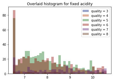
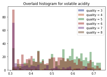
In the below graphs, we can see the distribution of data which would help us have a basic understanding of effects of different features on the quality of the wine.

# Check the distribution of data using histograms

sns.set_palette("dark")
features = list(wineMod.drop(['quality'], axis = 1).columns.values)
for i in features:
    quality3 = list(wineMod[wineMod['quality'] == 3][i].dropna())
    quality4 = list(wineMod[wineMod['quality'] == 4][i].dropna())
    quality5 = list(wineMod[wineMod['quality'] == 5][i].dropna())
    quality6 = list(wineMod[wineMod['quality'] == 6][i].dropna())
    quality7 = list(wineMod[wineMod['quality'] == 7][i].dropna())
    quality8 = list(wineMod[wineMod['quality'] == 8][i].dropna())
    xmin = min(min(quality3), min(quality4), min(quality5), min(quality6), min(quality7), min(quality8))
    xmax = max(max(quality3), max(quality4), max(quality5), max(quality6), max(quality7), max(quality8))
    width = (xmax - xmin) / 40
    sns.distplot(quality3, kde=False, bins=np.arange(xmin, xmax, width))
    sns.distplot(quality4, kde=False, bins=np.arange(xmin, xmax, width))
    sns.distplot(quality5, kde=False, bins=np.arange(xmin, xmax, width))
    sns.distplot(quality6, kde=False, bins=np.arange(xmin, xmax, width))
    sns.distplot(quality7, kde=False, bins=np.arange(xmin, xmax, width))
    sns.distplot(quality8, kde=False, bins=np.arange(xmin, xmax, width))
    plt.legend(['quality = 3', 'quality = 4', 'quality = 5', 'quality = 6', 'quality = 7', 'quality = 8'])
    plt.title('Overlaid histogram for {}'.format(i))
    plt.show()

png

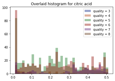
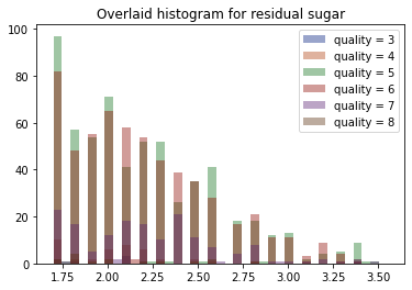
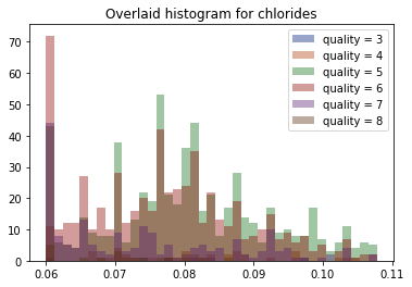
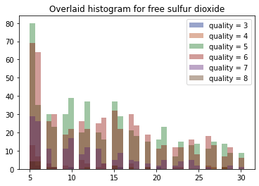
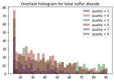
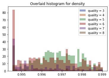
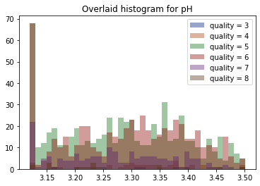
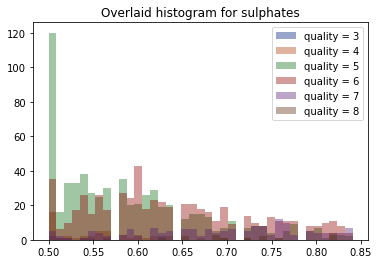
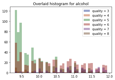
As we have mentioned earlier, the features are not on the same scale and we have class imbalance in our dataset. To fix this issue, we implement feature scaling by standard scalar.

# Prepare the data for modeling by carrying out any steps that you think are necessary
features = wineMod.drop('quality', axis=1)
labels = wineMod['quality']

# Creating Test and Train data
X_train, X_test, y_train, y_test = train_test_split(features, labels, test_size=0.2, random_state=42)

# implementing feature scaling
scaler = StandardScaler()
X_train = scaler.fit_transform(X_train)
X_test = scaler.transform(X_test)

Modeling

Implement Multivariable Linear Regression using any 2 Regression algorithms of your choice

Implement a Neural Network using Tensorflow and Keras to classify wine quality

# Implement Multivariable Linear Regression using any 2 Regression algorithms of your choice

# First Multivariable Linear Regression (Random Forest)
from sklearn.ensemble import RandomForestRegressor
rfModel = RandomForestRegressor(n_estimators=500)
rfModel.fit(X_train,y_train)
rfPreds = rfModel.predict(X_test)


# Second Multivariable Linear Regression Model (Gradient Boosting)
# We used GridSearchCV to find the best hyperparameters but as the output was large, we just used the hyperparameters we got from our GridSearch
from sklearn.ensemble import GradientBoostingRegressor

# parametersGb = {
#     "n_estimators":[5,50,250,500],
#     "max_depth":[1,3,5,7,9],
#     "learning_rate":[0.01,0.1,1,10,100]
# }
# gbGrid = GridSearchCV(GradientBoostingRegressor(), parametersGb, cv = 5)
# gbModel = gbGrid.fit(X_train, y_train)

gbModel = GradientBoostingRegressor(learning_rate=0.1, max_depth=3, n_estimators=250)
gbModel.fit(X_train,y_train)
gbPreds = gbModel.predict(X_test)

# Implement a Neural Network using Tensorflow and Keras to classify wine quality
import tensorflow as tf
tf.version.VERSION
from tensorflow import keras
from keras.models import Sequential
from keras.layers import Dense, Flatten

from tensorflow.keras.utils import to_categorical
from tensorflow.keras.optimizers import SGD

n_classes = 10
y_train_nn = to_categorical(y_train, n_classes)
y_test_nn = to_categorical(y_test, n_classes)

nnModel = Sequential()
nnModel.add(Dense(5, activation='relu', input_shape=(11,)))
nnModel.add(Dense(10, activation='softmax'))

nnModel.summary()

Model: "sequential"
_________________________________________________________________
Layer (type)                Output Shape              Param #   
=================================================================
dense (Dense)               (None, 5)                 60        
                                                                
dense_1 (Dense)             (None, 10)                60        
                                                                
=================================================================
Total params: 120
Trainable params: 120
Non-trainable params: 0
_________________________________________________________________

# Neural Network Model Configuration
nnModel.compile(loss='categorical_crossentropy', optimizer='adam', metrics=['accuracy'])

# Neural Network Model Training
history = nnModel.fit(X_train, y_train_nn, batch_size=128, epochs=200, verbose=1, validation_data=(X_test, y_test_nn))

Epoch 1/200
10/10 [==============================] - 1s 31ms/step - loss: 2.7089 - accuracy: 0.0868 - val_loss: 2.6831 - val_accuracy: 0.0938
Epoch 2/200
10/10 [==============================] - 0s 7ms/step - loss: 2.6298 - accuracy: 0.1032 - val_loss: 2.6036 - val_accuracy: 0.1125
Epoch 3/200
10/10 [==============================] - 0s 6ms/step - loss: 2.5549 - accuracy: 0.1235 - val_loss: 2.5281 - val_accuracy: 0.1562
Epoch 4/200
10/10 [==============================] - 0s 5ms/step - loss: 2.4843 - accuracy: 0.1540 - val_loss: 2.4571 - val_accuracy: 0.1750
Epoch 5/200
10/10 [==============================] - 0s 6ms/step - loss: 2.4177 - accuracy: 0.1775 - val_loss: 2.3905 - val_accuracy: 0.1937
Epoch 6/200
10/10 [==============================] - 0s 5ms/step - loss: 2.3565 - accuracy: 0.2064 - val_loss: 2.3276 - val_accuracy: 0.2094
Epoch 7/200
10/10 [==============================] - 0s 5ms/step - loss: 2.2982 - accuracy: 0.2103 - val_loss: 2.2691 - val_accuracy: 0.2125
Epoch 8/200
10/10 [==============================] - 0s 5ms/step - loss: 2.2441 - accuracy: 0.2252 - val_loss: 2.2146 - val_accuracy: 0.2219
Epoch 9/200
10/10 [==============================] - 0s 6ms/step - loss: 2.1933 - accuracy: 0.2392 - val_loss: 2.1642 - val_accuracy: 0.2313
Epoch 10/200
10/10 [==============================] - 0s 5ms/step - loss: 2.1463 - accuracy: 0.2518 - val_loss: 2.1169 - val_accuracy: 0.2562
Epoch 11/200
10/10 [==============================] - 0s 5ms/step - loss: 2.1020 - accuracy: 0.2619 - val_loss: 2.0731 - val_accuracy: 0.2781
Epoch 12/200
10/10 [==============================] - 0s 5ms/step - loss: 2.0617 - accuracy: 0.2682 - val_loss: 2.0312 - val_accuracy: 0.2812
Epoch 13/200
10/10 [==============================] - 0s 6ms/step - loss: 2.0218 - accuracy: 0.2760 - val_loss: 1.9930 - val_accuracy: 0.2812
Epoch 14/200
10/10 [==============================] - 0s 5ms/step - loss: 1.9855 - accuracy: 0.2932 - val_loss: 1.9562 - val_accuracy: 0.3000
Epoch 15/200
10/10 [==============================] - 0s 5ms/step - loss: 1.9502 - accuracy: 0.3159 - val_loss: 1.9221 - val_accuracy: 0.3063
Epoch 16/200
10/10 [==============================] - 0s 6ms/step - loss: 1.9170 - accuracy: 0.3339 - val_loss: 1.8896 - val_accuracy: 0.3281
Epoch 17/200
10/10 [==============================] - 0s 5ms/step - loss: 1.8856 - accuracy: 0.3487 - val_loss: 1.8586 - val_accuracy: 0.3469
Epoch 18/200
10/10 [==============================] - 0s 6ms/step - loss: 1.8556 - accuracy: 0.3698 - val_loss: 1.8293 - val_accuracy: 0.3656
Epoch 19/200
10/10 [==============================] - 0s 5ms/step - loss: 1.8267 - accuracy: 0.3831 - val_loss: 1.8012 - val_accuracy: 0.3781
Epoch 20/200
10/10 [==============================] - 0s 5ms/step - loss: 1.7988 - accuracy: 0.3980 - val_loss: 1.7745 - val_accuracy: 0.3875
Epoch 21/200
10/10 [==============================] - 0s 5ms/step - loss: 1.7727 - accuracy: 0.4081 - val_loss: 1.7483 - val_accuracy: 0.4031
Epoch 22/200
10/10 [==============================] - 0s 5ms/step - loss: 1.7468 - accuracy: 0.4128 - val_loss: 1.7237 - val_accuracy: 0.4156
Epoch 23/200
10/10 [==============================] - 0s 6ms/step - loss: 1.7223 - accuracy: 0.4206 - val_loss: 1.6999 - val_accuracy: 0.4281
Epoch 24/200
10/10 [==============================] - 0s 5ms/step - loss: 1.6986 - accuracy: 0.4269 - val_loss: 1.6767 - val_accuracy: 0.4344
Epoch 25/200
10/10 [==============================] - 0s 5ms/step - loss: 1.6760 - accuracy: 0.4324 - val_loss: 1.6539 - val_accuracy: 0.4406
Epoch 26/200
10/10 [==============================] - 0s 6ms/step - loss: 1.6541 - accuracy: 0.4355 - val_loss: 1.6318 - val_accuracy: 0.4469
Epoch 27/200
10/10 [==============================] - 0s 6ms/step - loss: 1.6329 - accuracy: 0.4418 - val_loss: 1.6104 - val_accuracy: 0.4625
Epoch 28/200
10/10 [==============================] - 0s 5ms/step - loss: 1.6125 - accuracy: 0.4433 - val_loss: 1.5899 - val_accuracy: 0.4625
Epoch 29/200
10/10 [==============================] - 0s 5ms/step - loss: 1.5924 - accuracy: 0.4441 - val_loss: 1.5705 - val_accuracy: 0.4500
Epoch 30/200
10/10 [==============================] - 0s 5ms/step - loss: 1.5737 - accuracy: 0.4480 - val_loss: 1.5516 - val_accuracy: 0.4531
Epoch 31/200
10/10 [==============================] - 0s 6ms/step - loss: 1.5551 - accuracy: 0.4527 - val_loss: 1.5333 - val_accuracy: 0.4594
Epoch 32/200
10/10 [==============================] - 0s 5ms/step - loss: 1.5375 - accuracy: 0.4597 - val_loss: 1.5156 - val_accuracy: 0.4750
Epoch 33/200
10/10 [==============================] - 0s 6ms/step - loss: 1.5201 - accuracy: 0.4629 - val_loss: 1.4989 - val_accuracy: 0.4750
Epoch 34/200
10/10 [==============================] - 0s 6ms/step - loss: 1.5038 - accuracy: 0.4652 - val_loss: 1.4826 - val_accuracy: 0.4781
Epoch 35/200
10/10 [==============================] - 0s 5ms/step - loss: 1.4872 - accuracy: 0.4707 - val_loss: 1.4668 - val_accuracy: 0.4750
Epoch 36/200
10/10 [==============================] - 0s 5ms/step - loss: 1.4714 - accuracy: 0.4722 - val_loss: 1.4511 - val_accuracy: 0.4781
Epoch 37/200
10/10 [==============================] - 0s 5ms/step - loss: 1.4558 - accuracy: 0.4801 - val_loss: 1.4351 - val_accuracy: 0.4938
Epoch 38/200
10/10 [==============================] - 0s 5ms/step - loss: 1.4400 - accuracy: 0.4855 - val_loss: 1.4198 - val_accuracy: 0.4938
Epoch 39/200
10/10 [==============================] - 0s 5ms/step - loss: 1.4243 - accuracy: 0.4902 - val_loss: 1.4049 - val_accuracy: 0.5031
Epoch 40/200
10/10 [==============================] - 0s 5ms/step - loss: 1.4094 - accuracy: 0.4934 - val_loss: 1.3901 - val_accuracy: 0.5031
Epoch 41/200
10/10 [==============================] - 0s 5ms/step - loss: 1.3939 - accuracy: 0.4980 - val_loss: 1.3760 - val_accuracy: 0.5094
Epoch 42/200
10/10 [==============================] - 0s 5ms/step - loss: 1.3795 - accuracy: 0.4988 - val_loss: 1.3620 - val_accuracy: 0.5125
Epoch 43/200
10/10 [==============================] - 0s 5ms/step - loss: 1.3648 - accuracy: 0.5082 - val_loss: 1.3487 - val_accuracy: 0.5281
Epoch 44/200
10/10 [==============================] - 0s 5ms/step - loss: 1.3510 - accuracy: 0.5106 - val_loss: 1.3358 - val_accuracy: 0.5250
Epoch 45/200
10/10 [==============================] - 0s 5ms/step - loss: 1.3374 - accuracy: 0.5168 - val_loss: 1.3231 - val_accuracy: 0.5281
Epoch 46/200
10/10 [==============================] - 0s 5ms/step - loss: 1.3244 - accuracy: 0.5223 - val_loss: 1.3108 - val_accuracy: 0.5250
Epoch 47/200
10/10 [==============================] - 0s 6ms/step - loss: 1.3120 - accuracy: 0.5223 - val_loss: 1.2989 - val_accuracy: 0.5281
Epoch 48/200
10/10 [==============================] - 0s 5ms/step - loss: 1.2999 - accuracy: 0.5262 - val_loss: 1.2877 - val_accuracy: 0.5250
Epoch 49/200
10/10 [==============================] - 0s 5ms/step - loss: 1.2889 - accuracy: 0.5285 - val_loss: 1.2767 - val_accuracy: 0.5250
Epoch 50/200
10/10 [==============================] - 0s 5ms/step - loss: 1.2776 - accuracy: 0.5285 - val_loss: 1.2659 - val_accuracy: 0.5312
Epoch 51/200
10/10 [==============================] - 0s 5ms/step - loss: 1.2664 - accuracy: 0.5309 - val_loss: 1.2560 - val_accuracy: 0.5375
Epoch 52/200
10/10 [==============================] - 0s 5ms/step - loss: 1.2564 - accuracy: 0.5364 - val_loss: 1.2460 - val_accuracy: 0.5375
Epoch 53/200
10/10 [==============================] - 0s 5ms/step - loss: 1.2459 - accuracy: 0.5395 - val_loss: 1.2367 - val_accuracy: 0.5469
Epoch 54/200
10/10 [==============================] - 0s 5ms/step - loss: 1.2362 - accuracy: 0.5395 - val_loss: 1.2278 - val_accuracy: 0.5406
Epoch 55/200
10/10 [==============================] - 0s 5ms/step - loss: 1.2270 - accuracy: 0.5410 - val_loss: 1.2191 - val_accuracy: 0.5406
Epoch 56/200
10/10 [==============================] - 0s 6ms/step - loss: 1.2176 - accuracy: 0.5442 - val_loss: 1.2108 - val_accuracy: 0.5406
Epoch 57/200
10/10 [==============================] - 0s 6ms/step - loss: 1.2089 - accuracy: 0.5465 - val_loss: 1.2028 - val_accuracy: 0.5406
Epoch 58/200
10/10 [==============================] - 0s 5ms/step - loss: 1.2001 - accuracy: 0.5450 - val_loss: 1.1953 - val_accuracy: 0.5375
Epoch 59/200
10/10 [==============================] - 0s 6ms/step - loss: 1.1919 - accuracy: 0.5442 - val_loss: 1.1878 - val_accuracy: 0.5375
Epoch 60/200
10/10 [==============================] - 0s 6ms/step - loss: 1.1840 - accuracy: 0.5481 - val_loss: 1.1808 - val_accuracy: 0.5375
Epoch 61/200
10/10 [==============================] - 0s 5ms/step - loss: 1.1763 - accuracy: 0.5504 - val_loss: 1.1738 - val_accuracy: 0.5406
Epoch 62/200
10/10 [==============================] - 0s 5ms/step - loss: 1.1689 - accuracy: 0.5559 - val_loss: 1.1669 - val_accuracy: 0.5500
Epoch 63/200
10/10 [==============================] - 0s 5ms/step - loss: 1.1618 - accuracy: 0.5582 - val_loss: 1.1602 - val_accuracy: 0.5531
Epoch 64/200
10/10 [==============================] - 0s 6ms/step - loss: 1.1548 - accuracy: 0.5629 - val_loss: 1.1540 - val_accuracy: 0.5531
Epoch 65/200
10/10 [==============================] - 0s 5ms/step - loss: 1.1479 - accuracy: 0.5653 - val_loss: 1.1480 - val_accuracy: 0.5531
Epoch 66/200
10/10 [==============================] - 0s 5ms/step - loss: 1.1412 - accuracy: 0.5684 - val_loss: 1.1425 - val_accuracy: 0.5594
Epoch 67/200
10/10 [==============================] - 0s 5ms/step - loss: 1.1350 - accuracy: 0.5715 - val_loss: 1.1372 - val_accuracy: 0.5625
Epoch 68/200
10/10 [==============================] - 0s 5ms/step - loss: 1.1289 - accuracy: 0.5739 - val_loss: 1.1321 - val_accuracy: 0.5625
Epoch 69/200
10/10 [==============================] - 0s 5ms/step - loss: 1.1230 - accuracy: 0.5754 - val_loss: 1.1271 - val_accuracy: 0.5656
Epoch 70/200
10/10 [==============================] - 0s 5ms/step - loss: 1.1174 - accuracy: 0.5794 - val_loss: 1.1224 - val_accuracy: 0.5656
Epoch 71/200
10/10 [==============================] - 0s 5ms/step - loss: 1.1119 - accuracy: 0.5809 - val_loss: 1.1183 - val_accuracy: 0.5719
Epoch 72/200
10/10 [==============================] - 0s 6ms/step - loss: 1.1067 - accuracy: 0.5825 - val_loss: 1.1144 - val_accuracy: 0.5688
Epoch 73/200
10/10 [==============================] - 0s 5ms/step - loss: 1.1018 - accuracy: 0.5817 - val_loss: 1.1106 - val_accuracy: 0.5719
Epoch 74/200
10/10 [==============================] - 0s 6ms/step - loss: 1.0972 - accuracy: 0.5817 - val_loss: 1.1069 - val_accuracy: 0.5750
Epoch 75/200
10/10 [==============================] - 0s 6ms/step - loss: 1.0929 - accuracy: 0.5825 - val_loss: 1.1035 - val_accuracy: 0.5656
Epoch 76/200
10/10 [==============================] - 0s 6ms/step - loss: 1.0884 - accuracy: 0.5825 - val_loss: 1.1001 - val_accuracy: 0.5625
Epoch 77/200
10/10 [==============================] - 0s 6ms/step - loss: 1.0843 - accuracy: 0.5833 - val_loss: 1.0969 - val_accuracy: 0.5594
Epoch 78/200
10/10 [==============================] - 0s 6ms/step - loss: 1.0805 - accuracy: 0.5825 - val_loss: 1.0939 - val_accuracy: 0.5594
Epoch 79/200
10/10 [==============================] - 0s 6ms/step - loss: 1.0766 - accuracy: 0.5817 - val_loss: 1.0909 - val_accuracy: 0.5562
Epoch 80/200
10/10 [==============================] - 0s 6ms/step - loss: 1.0730 - accuracy: 0.5872 - val_loss: 1.0880 - val_accuracy: 0.5562
Epoch 81/200
10/10 [==============================] - 0s 7ms/step - loss: 1.0693 - accuracy: 0.5864 - val_loss: 1.0850 - val_accuracy: 0.5625
Epoch 82/200
10/10 [==============================] - 0s 6ms/step - loss: 1.0660 - accuracy: 0.5817 - val_loss: 1.0820 - val_accuracy: 0.5625
Epoch 83/200
10/10 [==============================] - 0s 6ms/step - loss: 1.0626 - accuracy: 0.5833 - val_loss: 1.0790 - val_accuracy: 0.5656
Epoch 84/200
10/10 [==============================] - 0s 6ms/step - loss: 1.0594 - accuracy: 0.5848 - val_loss: 1.0760 - val_accuracy: 0.5719
Epoch 85/200
10/10 [==============================] - 0s 6ms/step - loss: 1.0562 - accuracy: 0.5903 - val_loss: 1.0728 - val_accuracy: 0.5750
Epoch 86/200
10/10 [==============================] - 0s 6ms/step - loss: 1.0530 - accuracy: 0.5911 - val_loss: 1.0701 - val_accuracy: 0.5781
Epoch 87/200
10/10 [==============================] - 0s 6ms/step - loss: 1.0504 - accuracy: 0.5934 - val_loss: 1.0672 - val_accuracy: 0.5781
Epoch 88/200
10/10 [==============================] - 0s 6ms/step - loss: 1.0473 - accuracy: 0.5950 - val_loss: 1.0645 - val_accuracy: 0.5781
Epoch 89/200
10/10 [==============================] - 0s 6ms/step - loss: 1.0446 - accuracy: 0.5973 - val_loss: 1.0617 - val_accuracy: 0.5750
Epoch 90/200
10/10 [==============================] - 0s 5ms/step - loss: 1.0420 - accuracy: 0.6005 - val_loss: 1.0590 - val_accuracy: 0.5750
Epoch 91/200
10/10 [==============================] - 0s 5ms/step - loss: 1.0393 - accuracy: 0.6013 - val_loss: 1.0565 - val_accuracy: 0.5813
Epoch 92/200
10/10 [==============================] - 0s 5ms/step - loss: 1.0367 - accuracy: 0.6028 - val_loss: 1.0541 - val_accuracy: 0.5781
Epoch 93/200
10/10 [==============================] - 0s 5ms/step - loss: 1.0344 - accuracy: 0.6020 - val_loss: 1.0518 - val_accuracy: 0.5750
Epoch 94/200
10/10 [==============================] - 0s 5ms/step - loss: 1.0319 - accuracy: 0.6013 - val_loss: 1.0495 - val_accuracy: 0.5750
Epoch 95/200
10/10 [==============================] - 0s 6ms/step - loss: 1.0295 - accuracy: 0.6013 - val_loss: 1.0474 - val_accuracy: 0.5719
Epoch 96/200
10/10 [==============================] - 0s 5ms/step - loss: 1.0274 - accuracy: 0.6028 - val_loss: 1.0453 - val_accuracy: 0.5719
Epoch 97/200
10/10 [==============================] - 0s 5ms/step - loss: 1.0254 - accuracy: 0.6036 - val_loss: 1.0430 - val_accuracy: 0.5719
Epoch 98/200
10/10 [==============================] - 0s 5ms/step - loss: 1.0232 - accuracy: 0.6036 - val_loss: 1.0411 - val_accuracy: 0.5719
Epoch 99/200
10/10 [==============================] - 0s 5ms/step - loss: 1.0212 - accuracy: 0.6020 - val_loss: 1.0392 - val_accuracy: 0.5656
Epoch 100/200
10/10 [==============================] - 0s 6ms/step - loss: 1.0194 - accuracy: 0.6036 - val_loss: 1.0371 - val_accuracy: 0.5625
Epoch 101/200
10/10 [==============================] - 0s 6ms/step - loss: 1.0174 - accuracy: 0.6052 - val_loss: 1.0352 - val_accuracy: 0.5625
Epoch 102/200
10/10 [==============================] - 0s 5ms/step - loss: 1.0156 - accuracy: 0.6052 - val_loss: 1.0334 - val_accuracy: 0.5594
Epoch 103/200
10/10 [==============================] - 0s 5ms/step - loss: 1.0137 - accuracy: 0.6067 - val_loss: 1.0316 - val_accuracy: 0.5625
Epoch 104/200
10/10 [==============================] - 0s 5ms/step - loss: 1.0119 - accuracy: 0.6067 - val_loss: 1.0299 - val_accuracy: 0.5656
Epoch 105/200
10/10 [==============================] - 0s 6ms/step - loss: 1.0102 - accuracy: 0.6083 - val_loss: 1.0280 - val_accuracy: 0.5656
Epoch 106/200
10/10 [==============================] - 0s 5ms/step - loss: 1.0085 - accuracy: 0.6075 - val_loss: 1.0261 - val_accuracy: 0.5656
Epoch 107/200
10/10 [==============================] - 0s 6ms/step - loss: 1.0067 - accuracy: 0.6067 - val_loss: 1.0244 - val_accuracy: 0.5688
Epoch 108/200
10/10 [==============================] - 0s 5ms/step - loss: 1.0049 - accuracy: 0.6059 - val_loss: 1.0228 - val_accuracy: 0.5750
Epoch 109/200
10/10 [==============================] - 0s 5ms/step - loss: 1.0032 - accuracy: 0.6052 - val_loss: 1.0212 - val_accuracy: 0.5781
Epoch 110/200
10/10 [==============================] - 0s 5ms/step - loss: 1.0017 - accuracy: 0.6059 - val_loss: 1.0194 - val_accuracy: 0.5750
Epoch 111/200
10/10 [==============================] - 0s 5ms/step - loss: 1.0001 - accuracy: 0.6075 - val_loss: 1.0178 - val_accuracy: 0.5750
Epoch 112/200
10/10 [==============================] - 0s 6ms/step - loss: 0.9986 - accuracy: 0.6083 - val_loss: 1.0165 - val_accuracy: 0.5750
Epoch 113/200
10/10 [==============================] - 0s 5ms/step - loss: 0.9970 - accuracy: 0.6106 - val_loss: 1.0150 - val_accuracy: 0.5781
Epoch 114/200
10/10 [==============================] - 0s 5ms/step - loss: 0.9955 - accuracy: 0.6106 - val_loss: 1.0135 - val_accuracy: 0.5813
Epoch 115/200
10/10 [==============================] - 0s 5ms/step - loss: 0.9940 - accuracy: 0.6099 - val_loss: 1.0119 - val_accuracy: 0.5813
Epoch 116/200
10/10 [==============================] - 0s 5ms/step - loss: 0.9925 - accuracy: 0.6099 - val_loss: 1.0104 - val_accuracy: 0.5781
Epoch 117/200
10/10 [==============================] - 0s 5ms/step - loss: 0.9911 - accuracy: 0.6075 - val_loss: 1.0088 - val_accuracy: 0.5781
Epoch 118/200
10/10 [==============================] - 0s 5ms/step - loss: 0.9897 - accuracy: 0.6083 - val_loss: 1.0072 - val_accuracy: 0.5781
Epoch 119/200
10/10 [==============================] - 0s 5ms/step - loss: 0.9883 - accuracy: 0.6067 - val_loss: 1.0058 - val_accuracy: 0.5719
Epoch 120/200
10/10 [==============================] - 0s 6ms/step - loss: 0.9869 - accuracy: 0.6067 - val_loss: 1.0043 - val_accuracy: 0.5719
Epoch 121/200
10/10 [==============================] - 0s 5ms/step - loss: 0.9854 - accuracy: 0.6067 - val_loss: 1.0030 - val_accuracy: 0.5719
Epoch 122/200
10/10 [==============================] - 0s 5ms/step - loss: 0.9841 - accuracy: 0.6075 - val_loss: 1.0018 - val_accuracy: 0.5719
Epoch 123/200
10/10 [==============================] - 0s 5ms/step - loss: 0.9827 - accuracy: 0.6052 - val_loss: 1.0005 - val_accuracy: 0.5719
Epoch 124/200
10/10 [==============================] - 0s 5ms/step - loss: 0.9815 - accuracy: 0.6044 - val_loss: 0.9992 - val_accuracy: 0.5688
Epoch 125/200
10/10 [==============================] - 0s 5ms/step - loss: 0.9802 - accuracy: 0.6028 - val_loss: 0.9978 - val_accuracy: 0.5656
Epoch 126/200
10/10 [==============================] - 0s 6ms/step - loss: 0.9791 - accuracy: 0.6028 - val_loss: 0.9964 - val_accuracy: 0.5625
Epoch 127/200
10/10 [==============================] - 0s 5ms/step - loss: 0.9778 - accuracy: 0.6020 - val_loss: 0.9953 - val_accuracy: 0.5656
Epoch 128/200
10/10 [==============================] - 0s 5ms/step - loss: 0.9767 - accuracy: 0.6013 - val_loss: 0.9940 - val_accuracy: 0.5656
Epoch 129/200
10/10 [==============================] - 0s 5ms/step - loss: 0.9756 - accuracy: 0.5997 - val_loss: 0.9927 - val_accuracy: 0.5688
Epoch 130/200
10/10 [==============================] - 0s 5ms/step - loss: 0.9743 - accuracy: 0.5997 - val_loss: 0.9914 - val_accuracy: 0.5688
Epoch 131/200
10/10 [==============================] - 0s 5ms/step - loss: 0.9734 - accuracy: 0.5997 - val_loss: 0.9901 - val_accuracy: 0.5688
Epoch 132/200
10/10 [==============================] - 0s 5ms/step - loss: 0.9723 - accuracy: 0.5981 - val_loss: 0.9889 - val_accuracy: 0.5688
Epoch 133/200
10/10 [==============================] - 0s 5ms/step - loss: 0.9712 - accuracy: 0.5973 - val_loss: 0.9876 - val_accuracy: 0.5719
Epoch 134/200
10/10 [==============================] - 0s 5ms/step - loss: 0.9702 - accuracy: 0.5973 - val_loss: 0.9865 - val_accuracy: 0.5688
Epoch 135/200
10/10 [==============================] - 0s 5ms/step - loss: 0.9691 - accuracy: 0.5973 - val_loss: 0.9854 - val_accuracy: 0.5719
Epoch 136/200
10/10 [==============================] - 0s 5ms/step - loss: 0.9682 - accuracy: 0.5981 - val_loss: 0.9843 - val_accuracy: 0.5719
Epoch 137/200
10/10 [==============================] - 0s 5ms/step - loss: 0.9672 - accuracy: 0.5973 - val_loss: 0.9833 - val_accuracy: 0.5688
Epoch 138/200
10/10 [==============================] - 0s 5ms/step - loss: 0.9662 - accuracy: 0.5973 - val_loss: 0.9821 - val_accuracy: 0.5719
Epoch 139/200
10/10 [==============================] - 0s 5ms/step - loss: 0.9654 - accuracy: 0.5966 - val_loss: 0.9809 - val_accuracy: 0.5813
Epoch 140/200
10/10 [==============================] - 0s 5ms/step - loss: 0.9644 - accuracy: 0.6005 - val_loss: 0.9799 - val_accuracy: 0.5813
Epoch 141/200
10/10 [==============================] - 0s 5ms/step - loss: 0.9635 - accuracy: 0.5989 - val_loss: 0.9790 - val_accuracy: 0.5781
Epoch 142/200
10/10 [==============================] - 0s 5ms/step - loss: 0.9627 - accuracy: 0.5958 - val_loss: 0.9777 - val_accuracy: 0.5750
Epoch 143/200
10/10 [==============================] - 0s 5ms/step - loss: 0.9618 - accuracy: 0.5942 - val_loss: 0.9764 - val_accuracy: 0.5719
Epoch 144/200
10/10 [==============================] - 0s 5ms/step - loss: 0.9610 - accuracy: 0.5934 - val_loss: 0.9754 - val_accuracy: 0.5781
Epoch 145/200
10/10 [==============================] - 0s 5ms/step - loss: 0.9601 - accuracy: 0.5950 - val_loss: 0.9745 - val_accuracy: 0.5813
Epoch 146/200
10/10 [==============================] - 0s 6ms/step - loss: 0.9594 - accuracy: 0.5942 - val_loss: 0.9734 - val_accuracy: 0.5813
Epoch 147/200
10/10 [==============================] - 0s 6ms/step - loss: 0.9586 - accuracy: 0.5934 - val_loss: 0.9724 - val_accuracy: 0.5781
Epoch 148/200
10/10 [==============================] - 0s 5ms/step - loss: 0.9578 - accuracy: 0.5934 - val_loss: 0.9715 - val_accuracy: 0.5781
Epoch 149/200
10/10 [==============================] - 0s 5ms/step - loss: 0.9572 - accuracy: 0.5934 - val_loss: 0.9705 - val_accuracy: 0.5781
Epoch 150/200
10/10 [==============================] - 0s 6ms/step - loss: 0.9564 - accuracy: 0.5950 - val_loss: 0.9696 - val_accuracy: 0.5781
Epoch 151/200
10/10 [==============================] - 0s 5ms/step - loss: 0.9557 - accuracy: 0.5942 - val_loss: 0.9689 - val_accuracy: 0.5781
Epoch 152/200
10/10 [==============================] - 0s 5ms/step - loss: 0.9549 - accuracy: 0.5942 - val_loss: 0.9679 - val_accuracy: 0.5750
Epoch 153/200
10/10 [==============================] - 0s 5ms/step - loss: 0.9542 - accuracy: 0.5958 - val_loss: 0.9671 - val_accuracy: 0.5750
Epoch 154/200
10/10 [==============================] - 0s 5ms/step - loss: 0.9535 - accuracy: 0.5950 - val_loss: 0.9662 - val_accuracy: 0.5719
Epoch 155/200
10/10 [==============================] - 0s 5ms/step - loss: 0.9529 - accuracy: 0.5934 - val_loss: 0.9654 - val_accuracy: 0.5750
Epoch 156/200
10/10 [==============================] - 0s 5ms/step - loss: 0.9522 - accuracy: 0.5927 - val_loss: 0.9645 - val_accuracy: 0.5719
Epoch 157/200
10/10 [==============================] - 0s 5ms/step - loss: 0.9516 - accuracy: 0.5942 - val_loss: 0.9638 - val_accuracy: 0.5750
Epoch 158/200
10/10 [==============================] - 0s 5ms/step - loss: 0.9509 - accuracy: 0.5919 - val_loss: 0.9630 - val_accuracy: 0.5750
Epoch 159/200
10/10 [==============================] - 0s 5ms/step - loss: 0.9502 - accuracy: 0.5895 - val_loss: 0.9621 - val_accuracy: 0.5750
Epoch 160/200
10/10 [==============================] - 0s 5ms/step - loss: 0.9496 - accuracy: 0.5903 - val_loss: 0.9612 - val_accuracy: 0.5719
Epoch 161/200
10/10 [==============================] - 0s 5ms/step - loss: 0.9489 - accuracy: 0.5903 - val_loss: 0.9604 - val_accuracy: 0.5719
Epoch 162/200
10/10 [==============================] - 0s 5ms/step - loss: 0.9483 - accuracy: 0.5934 - val_loss: 0.9596 - val_accuracy: 0.5750
Epoch 163/200
10/10 [==============================] - 0s 5ms/step - loss: 0.9478 - accuracy: 0.5950 - val_loss: 0.9588 - val_accuracy: 0.5781
Epoch 164/200
10/10 [==============================] - 0s 5ms/step - loss: 0.9471 - accuracy: 0.5958 - val_loss: 0.9580 - val_accuracy: 0.5781
Epoch 165/200
10/10 [==============================] - 0s 6ms/step - loss: 0.9464 - accuracy: 0.5966 - val_loss: 0.9571 - val_accuracy: 0.5781
Epoch 166/200
10/10 [==============================] - 0s 6ms/step - loss: 0.9459 - accuracy: 0.5958 - val_loss: 0.9564 - val_accuracy: 0.5781
Epoch 167/200
10/10 [==============================] - 0s 6ms/step - loss: 0.9454 - accuracy: 0.5958 - val_loss: 0.9556 - val_accuracy: 0.5781
Epoch 168/200
10/10 [==============================] - 0s 6ms/step - loss: 0.9450 - accuracy: 0.5942 - val_loss: 0.9549 - val_accuracy: 0.5781
Epoch 169/200
10/10 [==============================] - 0s 6ms/step - loss: 0.9444 - accuracy: 0.5942 - val_loss: 0.9542 - val_accuracy: 0.5813
Epoch 170/200
10/10 [==============================] - 0s 6ms/step - loss: 0.9439 - accuracy: 0.5966 - val_loss: 0.9535 - val_accuracy: 0.5844
Epoch 171/200
10/10 [==============================] - 0s 6ms/step - loss: 0.9434 - accuracy: 0.5950 - val_loss: 0.9530 - val_accuracy: 0.5844
Epoch 172/200
10/10 [==============================] - 0s 6ms/step - loss: 0.9428 - accuracy: 0.5942 - val_loss: 0.9522 - val_accuracy: 0.5844
Epoch 173/200
10/10 [==============================] - 0s 5ms/step - loss: 0.9424 - accuracy: 0.5942 - val_loss: 0.9514 - val_accuracy: 0.5844
Epoch 174/200
10/10 [==============================] - 0s 6ms/step - loss: 0.9417 - accuracy: 0.5927 - val_loss: 0.9507 - val_accuracy: 0.5844
Epoch 175/200
10/10 [==============================] - 0s 6ms/step - loss: 0.9413 - accuracy: 0.5927 - val_loss: 0.9498 - val_accuracy: 0.5938
Epoch 176/200
10/10 [==============================] - 0s 5ms/step - loss: 0.9409 - accuracy: 0.5942 - val_loss: 0.9491 - val_accuracy: 0.5875
Epoch 177/200
10/10 [==============================] - 0s 6ms/step - loss: 0.9403 - accuracy: 0.5927 - val_loss: 0.9486 - val_accuracy: 0.5938
Epoch 178/200
10/10 [==============================] - 0s 6ms/step - loss: 0.9399 - accuracy: 0.5934 - val_loss: 0.9480 - val_accuracy: 0.5969
Epoch 179/200
10/10 [==============================] - 0s 6ms/step - loss: 0.9394 - accuracy: 0.5934 - val_loss: 0.9473 - val_accuracy: 0.5938
Epoch 180/200
10/10 [==============================] - 0s 6ms/step - loss: 0.9390 - accuracy: 0.5942 - val_loss: 0.9469 - val_accuracy: 0.5969
Epoch 181/200
10/10 [==============================] - 0s 6ms/step - loss: 0.9386 - accuracy: 0.5942 - val_loss: 0.9463 - val_accuracy: 0.5906
Epoch 182/200
10/10 [==============================] - 0s 6ms/step - loss: 0.9381 - accuracy: 0.5966 - val_loss: 0.9457 - val_accuracy: 0.5969
Epoch 183/200
10/10 [==============================] - 0s 5ms/step - loss: 0.9377 - accuracy: 0.5966 - val_loss: 0.9451 - val_accuracy: 0.5938
Epoch 184/200
10/10 [==============================] - 0s 5ms/step - loss: 0.9374 - accuracy: 0.5958 - val_loss: 0.9448 - val_accuracy: 0.5906
Epoch 185/200
10/10 [==============================] - 0s 5ms/step - loss: 0.9368 - accuracy: 0.6005 - val_loss: 0.9442 - val_accuracy: 0.5938
Epoch 186/200
10/10 [==============================] - 0s 5ms/step - loss: 0.9364 - accuracy: 0.5981 - val_loss: 0.9434 - val_accuracy: 0.6000
Epoch 187/200
10/10 [==============================] - 0s 6ms/step - loss: 0.9358 - accuracy: 0.5973 - val_loss: 0.9429 - val_accuracy: 0.5969
Epoch 188/200
10/10 [==============================] - 0s 5ms/step - loss: 0.9354 - accuracy: 0.5981 - val_loss: 0.9422 - val_accuracy: 0.5938
Epoch 189/200
10/10 [==============================] - 0s 6ms/step - loss: 0.9350 - accuracy: 0.5981 - val_loss: 0.9415 - val_accuracy: 0.5969
Epoch 190/200
10/10 [==============================] - 0s 5ms/step - loss: 0.9346 - accuracy: 0.5981 - val_loss: 0.9412 - val_accuracy: 0.5969
Epoch 191/200
10/10 [==============================] - 0s 5ms/step - loss: 0.9342 - accuracy: 0.5989 - val_loss: 0.9407 - val_accuracy: 0.5969
Epoch 192/200
10/10 [==============================] - 0s 5ms/step - loss: 0.9336 - accuracy: 0.6013 - val_loss: 0.9399 - val_accuracy: 0.5969
Epoch 193/200
10/10 [==============================] - 0s 5ms/step - loss: 0.9332 - accuracy: 0.6020 - val_loss: 0.9395 - val_accuracy: 0.5969
Epoch 194/200
10/10 [==============================] - 0s 5ms/step - loss: 0.9329 - accuracy: 0.6005 - val_loss: 0.9390 - val_accuracy: 0.5969
Epoch 195/200
10/10 [==============================] - 0s 6ms/step - loss: 0.9325 - accuracy: 0.6020 - val_loss: 0.9383 - val_accuracy: 0.5969
Epoch 196/200
10/10 [==============================] - 0s 5ms/step - loss: 0.9321 - accuracy: 0.6020 - val_loss: 0.9378 - val_accuracy: 0.5938
Epoch 197/200
10/10 [==============================] - 0s 5ms/step - loss: 0.9318 - accuracy: 0.6013 - val_loss: 0.9371 - val_accuracy: 0.5938
Epoch 198/200
10/10 [==============================] - 0s 6ms/step - loss: 0.9311 - accuracy: 0.6036 - val_loss: 0.9367 - val_accuracy: 0.5938
Epoch 199/200
10/10 [==============================] - 0s 5ms/step - loss: 0.9309 - accuracy: 0.6044 - val_loss: 0.9359 - val_accuracy: 0.5938
Epoch 200/200
10/10 [==============================] - 0s 5ms/step - loss: 0.9304 - accuracy: 0.6052 - val_loss: 0.9355 - val_accuracy: 0.5938

Model Evaluation

Evaluating the model accuracy is an essential part of the process in creating machine learning models to describe how well the model is performing in its predictions. Evaluation metrics change according to the problem type. Here, we’ll briefly learn how to check the accuracy of the regression model.

The linear model (regression) can be a typical example of this type of problem, and the main characteristic of the regression problem is that the targets of a dataset contain the real numbers only. The errors represent how much the model is making mistakes in its prediction. The basic concept of accuracy evaluation is to compare the original target with the predicted one according to certain metrics.

Regression model evaluation metrics

The MAE, RMSE, and R-Squared metrics are mainly used to evaluate the prediction error rates and model performance in regression analysis.

MAE (Mean absolute error) represents the difference between the original and predicted values extracted by averaged the absolute difference over the data set.

RMSE (Root Mean Squared Error) is the error rate by the square root of MSE.

R-squared (Coefficient of determination) represents the coefficient of how well the values fit compared to the original values. The value from 0 to 1 interpreted as percentages. The higher the value is, the better the model is.

The above metrics can be expressed as following: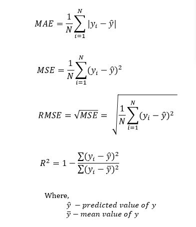

Please find more information on how to implement them from this link: https://scikit-learn.org/stable/modules/classes.html#regression-metrics

Find more about feature importances from here: https://machinelearningmastery.com/calculate-feature-importance-with-python/

Classification model evaluation metrics

For Regression models

Use three metrics: R-squared, RMSE, and MAE, to evaluate model prediction performance

Compare these 3 metrics for the two models and analyze the performance

Calculate the feature importance scores for the top features that help predicting wine quality and visualize them

For Classification model

Plot training loss and validation loss

Plot training accuracy and validation accuracy

Evaluate the classsification model using Precision, Recall and Accuracy metrics

Evaluation of Regression models

The Random Forest model has better scores in all of the R^2, RMSE, and MAE than the Gradient Boosting model as it is shown below. Random Forest model has R^2 of 0.53 whereas the Gradient Boosting model’s R^2 is 0.49 (the higher, the better). Random forest has RMSE and MAE of 0.56, and 0.42, respectively, whereas the Gradient Boosting model has RMSE and MAE of 0.58, and 0.45 (the lower, the better).

from sklearn.metrics import mean_absolute_error, r2_score, mean_squared_error
from math import sqrt

def r2(y_, y):
    return r2_score(y_, y)
def rmse(y_, y):
    return sqrt(mean_squared_error(y_, y))
def mae(y_, y):
    return mean_absolute_error(y_, y)

print('Random Forest scores: R^2: {}, RMSE: {}, MAE: {}'.format(r2(y_test, rfPreds), rmse(y_test, rfPreds), mae(y_test, rfPreds)))
print('Gradient Boosting scores: R^2: {}, RMSE: {}, MAE: {}'.format(r2(y_test, gbPreds), rmse(y_test, gbPreds), mae(y_test, gbPreds)))

Random Forest scores: R^2: 0.5237219061850895, RMSE: 0.5578983106265872, MAE: 0.42939999999999995
Gradient Boosting scores: R^2: 0.48972586316712086, RMSE: 0.5774661360701656, MAE: 0.4515129888215445

As we can see from the below graphs, both of our regression models, had almost the same determination for features’ importance. The highest feature importance is related to the alcohol feature which was predictable as the alcohol had the highest correlation with the wine’s quality.

# Calculating feature importance
from matplotlib import pyplot

rfImportance = rfModel.feature_importances_
gbImportance = gbModel.feature_importances_

featuresNames = list(wineMod.columns)
# summarize feature importance
print("Random Forest Regression Feature Importance: ")
for i,v in enumerate(rfImportance):
    print('Feature: %20s, Score: %.5f' % (featuresNames[i],v))

print("\n\nGradient Boosting Regression Feature Importance: ")
for i,v in enumerate(gbImportance):
    print('Feature: %20s, Score: %.5f' % (featuresNames[i],v))

# plot feature importance
print("\n\nRandom Forest Regression Feature Importance Plot: ")
pyplot.figure(figsize=(20, 3))
pyplot.bar(featuresNames[:-1], list(rfImportance))
pyplot.show()

print("\n\nGradient Boosting Regression Feature Importance Plot: ")
pyplot.figure(figsize=(20, 3))
pyplot.bar(featuresNames[:-1], list(gbImportance))
pyplot.show()

Random Forest Regression Feature Importance: 
Feature:        fixed acidity, Score: 0.05458
Feature:     volatile acidity, Score: 0.09749
Feature:          citric acid, Score: 0.05529
Feature:       residual sugar, Score: 0.04788
Feature:            chlorides, Score: 0.06904
Feature:  free sulfur dioxide, Score: 0.05178
Feature: total sulfur dioxide, Score: 0.08317
Feature:              density, Score: 0.05652
Feature:                   pH, Score: 0.05768
Feature:            sulphates, Score: 0.15882
Feature:              alcohol, Score: 0.26774


Gradient Boosting Regression Feature Importance: 
Feature:        fixed acidity, Score: 0.06297
Feature:     volatile acidity, Score: 0.10438
Feature:          citric acid, Score: 0.04191
Feature:       residual sugar, Score: 0.02639
Feature:            chlorides, Score: 0.06071
Feature:  free sulfur dioxide, Score: 0.03230
Feature: total sulfur dioxide, Score: 0.08289
Feature:              density, Score: 0.05654
Feature:                   pH, Score: 0.05041
Feature:            sulphates, Score: 0.17765
Feature:              alcohol, Score: 0.30386


Random Forest Regression Feature Importance Plot: 

png

Gradient Boosting Regression Feature Importance Plot:

png

Evaluation of Classification model

As we can see from the below graphs, our Neural Network performs how it should perform meaning that our model did not overfit, or underfit the training data and we have almost the same accuracy scores for both of train and test sets. The training loss and test loss are the same too meaning that the model’s loss would be around the same for the unseen data.

# Got this code from Stack Overflow
plt.plot(history.history['accuracy'])
plt.plot(history.history['val_accuracy'])
plt.title('Training Accuracy Vs. Validation Accuracy')
plt.ylabel('accuracy')
plt.xlabel('epoch')
plt.legend(['train', 'test'], loc='upper left')
plt.show()

plt.plot(history.history['loss'])
plt.plot(history.history['val_loss'])
plt.title('Training loss Vs. Validation loss')
plt.ylabel('loss')
plt.xlabel('epoch')
plt.legend(['train', 'val'], loc='upper left')
plt.show()

png

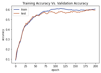
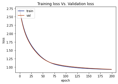
The Neural Network model we have trained, has the scores of:

Accuracy: 0.59
Precision (weighted): 0.56
Recall (weighted): 0.59

y_predict = nnModel.predict(X_test)
y_predict_num = np.argmax(y_predict, axis=1)

# Got this code from https://machinelearningmastery.com/how-to-calculate-precision-recall-f1-and-more-for-deep-learning-models/
# accuracy: (tp + tn) / (p + n)
accuracy = accuracy_score(y_test, y_predict_num)
print('Accuracy: %f' % accuracy)
# precision tp / (tp + fp)
precision = precision_score(y_test, y_predict_num, average='weighted')
print('Precision: %f' % precision)
# recall: tp / (tp + fn)
recall = recall_score(y_test, y_predict_num, average='weighted')
print('Recall: %f' % recall)

Accuracy: 0.593750
Precision: 0.559540
Recall: 0.593750

Conclusion

The scores of our regression models:

Random Forest scores:
- R^2: 0.52
- RMSE: 0.56
- MAE: 0.43
Gradient Boosting scores:
- R^2: 0.49
- RMSE: 0.58
- MAE: 0.45

The scores of our classification model (NN):

Accuracy: 0.59
Precision: 0.56
Recall: 0.59

By comparing the performance scores, we can conclude that the Neural Network model performs much better than the other two regression models. Since the wine quality dataset contains lots of features and moderate correlations between many of the features, the relationships between different attributes of the dataset is hard to obtain and regression models are not good at finding complex relationships. But, the Neural Network models can be very useful to obtain these relationships as they are very good at very complex tasks. However, the Neural Network models need a very large amount of data which we do not have and due to that our classification model’s performance scores were not as high as it could have been.

Amirhossein Razavi

Overview

Methodology

Evaluation

Key Findings

Personal Contributions

Conclusion

Project’s Jupyter Notebook

Exploring Red Wine Quality Through Data Science

Business Understanding

Analytic Approach

Data Requirements

Data Collection

Data Understanding

Data Preparation

Explore the dataset further

Modeling

Model Evaluation

Evaluation of Regression models

Evaluation of Classification model

Conclusion